This is a Kaggle competition with the task of detecting vehicles or obstacles in radar signals recorded by road vehicles. The training set consists of 15500 images with 55x128 pixels.
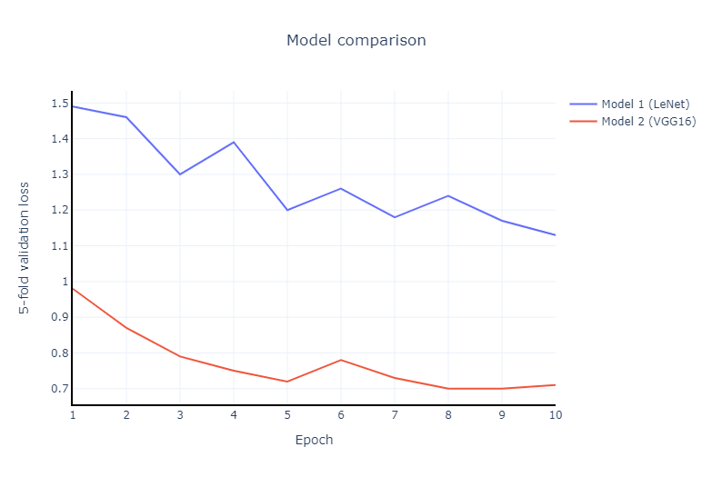
I tried two CNN models to solve the task. The first one, with a simple architecture inspired by LeNet, had at most 54% validation accuracy. It didn’t get a great accuracy, but it was fast to implement and fast to train. The second model, similar to VGG16, had at most 75% validation accuracy (for a single model, not the final ensemble) and was used for making the Kaggle submissions.
The training set was augmented with images flipped horizontally, vertically, horizontally and vertically. The validation set was not changed. Data augmentation improved the model performance a lot, even if training time slowed down significantly.
For splitting data into training and validation, both k-fold split and random split were implemented. K-fold was used for collecting results in the tables below. A seed was used to have reproducible fold configurations. However, I preferred using random split for making the submissions because it was easier to choose the train and validation sizes. A splitting of 14000-1500 (90.3% - 9.7%) worked fine.
The data was normalized and standardized.
Batch sizes of 32 had the best results, 64 slightly worse, 128 impossible to run on my device due to running out of CUDA memory.
A learning rate of 0.0001 seems the most stable without sacrificing too much training time. Learning rates 0.1, 0.01, 0.001 etc. were also tested.
The best activation function found is ReLU. Sigmoid and Softplus had worse results.
Fully connected layers have a 25% dropout to reduce overfitting. Dropout on convolutional layers was also tried, but it negatively impacted the model performance.
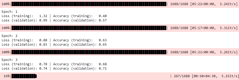
Average cross entropy loss and accuracy get calculated for training and validation at each epoch. The model gets saved if it has the highest validation accuracy found. After training is complete, the best model is loaded to make predictions on test data.
An homogenous ensemble of 5 models is used for hard voting on the final predictions.
Architecture of the first model tried, inspired by LeNet:
- Convolutional layer with kernel 5, stride 1, padding 0, batch normalization, ReLU
- Average pooling with kernel 2, stride 2, padding 0
- Convolutional layer with kernel 5, stride 1, padding 0, batch normalization, ReLU
- Average pooling with kernel 2, stride 2, padding 0
- Fully connected layer with input size 9280, dropout 25%
- Fully connected layer with input size 512, dropout 25%
- Fully connected layer with input size 64, output size 5
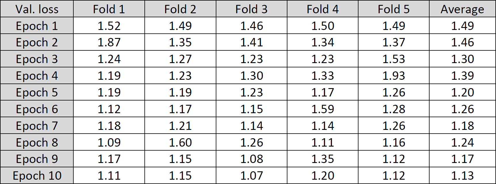
Validation cross entropy loss per epoch for each fold:
Architecture of the second model tried, inspired by VGG16:
- Convolutional layer with kernel 3, stride 1, padding 1, batch normalization, ReLU
- Convolutional layer with kernel 3, stride 1, padding 1, batch normalization, ReLU
- Max pooling with kernel 2, stride 2, padding 0
- Convolutional layer (same as above)
- Convolutional layer
- Max pooling
- Convolutional layer
- Convolutional layer
- Convolutional layer
- Convolutional layer
- Max pooling
- Convolutional layer
- Convolutional layer
- Convolutional layer
- Convolutional layer
- Max pooling
- Fully connected layer with input size 6144, dropout 25%
- Fully connected layer with input size 512, dropout 25%
- Fully connected layer with input size 64, output size 5
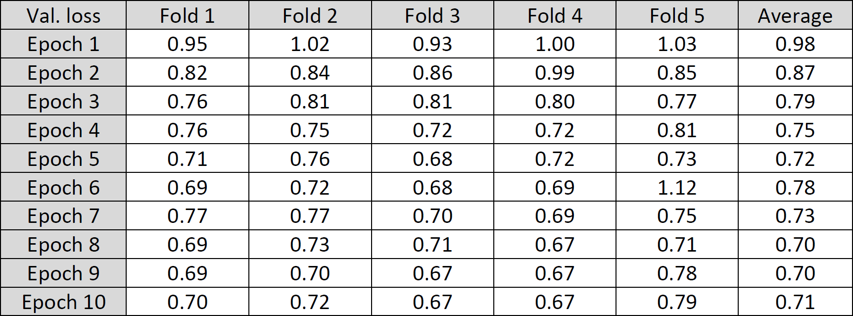
Validation cross entropy loss per epoch for each fold:
A comparison of the models’ average cross entropy loss (data from tables above):
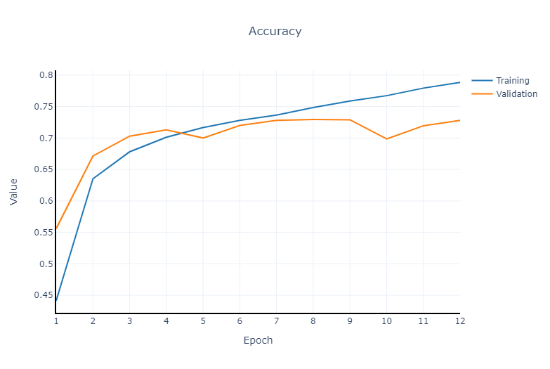
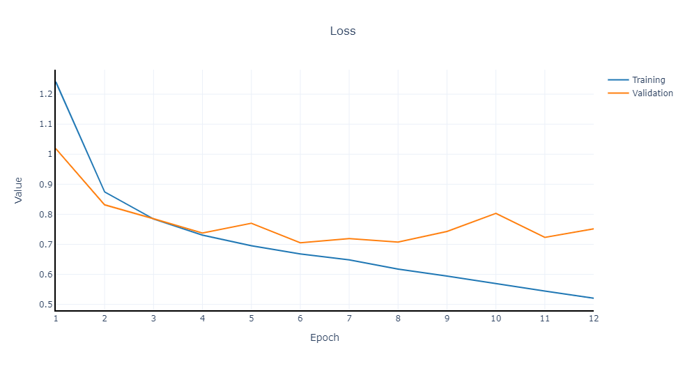
Accuracy and loss plots get generated at each run. Example of a 12 epochs run:
Model training info:
Source code is here.